Description of the method used¶

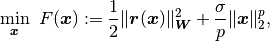
RALFit computes a solution $\vx$ to the non-linear least-squares problem

(1)¶ $\min_\vx \ F(\vx) := \frac{1}{2}\| \vr(\vx) \|_{\vW}^2 + \frac{\sigma}{p}\| \vx\|_2^p,$

Here we describe the method used to solve (1). RALFit implements an iterative method that, at each iteration, calculates and returns a step $\vs$ that reduces the model by an acceptable amount by solving (or approximating a solution to) a subproblem, as detailed in Subproblem solves.

The algorithm is iterative. At each point, $\iter{\vx}$ , the algorithm builds a model of the function at the next step, $F({\iter{\vx}+\iter{\vs}})$ , which we refer to as $m_k(\cdot)$ . We allow either a Gauss-Newton model, a (quasi-)Newton model, or a Newton-tensor model; see The models for more details.

Once the model has been formed we find a candidate for the next step by solving a subitable subproblem. The quantity

(2)¶ $\rho = \frac{F(\iter{\vx}) - F(\iter{\vx} + \iter{\vs})}{\iter{m}(\iter{\vx}) - \iter{m}(\iter{\vx} + \iter{\vs})}$

is then calculated. If this is sufficiently large we accept the step, and $\iter[k+1]{\vx}$ is set to $\iter{\vx} + \iter{\vs}$ ; if not, the parameter $\Delta_k$ is reduced and the resulting new trust-region sub-problem is solved. If the step is very successful – in that $\rho$ is close to one – $\Delta_k$ is increased. Details are explained in Accepting the step and updating the parameter.

This process continues until either the residual, $\|\vr(\iter{\vx})\|_\vW$ , or a measure of the gradient, $\|{\iter{\vJ}}^T\vW\vr(\iter{\vx})\|_2 / \|\vr(\iter{\vx})\|_\vW$ , is sufficiently small.

The models¶

A vital component of the algorithm is the choice of model employed. There are four choices available, controlled by the parameter model of nlls_options.

model = 1

this implements the Gauss-Newton model. Here we replace $\vr(\iter[k]{\vx} + \vs)$ by its first-order Taylor approximation, $\vr(\iter{\vx}) + \iter{\vJ}\vs$ . The model is therefore given by

(3)¶ $m_k^{GN}(\vs) = \frac{1}{2} \|\vr(\iter{\vx}) + \iter{\vJ}\vs\|_\vW^2.$

model = 2

this implements the Newton model. Here, instead of approximating the residual, $\vr(\cdot)$ , we take as our model the second-order Taylor approximation of the function, $F(\iter[k+1]{\vx}).$ Namely, we use

(4)¶

where $\iter{\vg} = {\iter{\vJ}}^T\vW \vr(\iter{\vx})$ and $\iter{\vH} = \sum_{i=1}^m\iter[i]{r}(\iter{\vx}) \vW \nabla^2 \iter[i]{r}(\iter{\vx}).$ Note that $m_k^{N}(\vs) = m_k^{GN}(\vs) + \frac{1}{2}\vs^T\iter{\vH} \vs$ .

If the second derivatives of $\vr(\cdot)$ are not available (i.e., the option exact_second_derivatives is set to false, then the method approximates the matrix $\iter{\vH}$ ; see Approximating the Hessian.

model = 3

This implements a hybrid model. In practice the Gauss-Newton model tends to work well far away from the solution, whereas Newton performs better once we are near to the minimum (particularly if the residual is large at the solution). This option will try to switch between these two models, picking the model that is most appropriate for the step. In particular, we start using $m_k^{GN}(\cdot)$ , and switch to $m_k^{N}(\cdot)$ if $\|{\iter{\vg}}\|_2 \leq \mathtt{hybrid\_tol} \frac{1}{2}\|\vr(\iter{\vx})\|^2_\vW$ for more than hybrid_switch_its iterations in a row. If, in subsequent iterations, we fail to get a decrease in the function value, then the algorithm interprets this as being not sufficiently close to the solution, and thus switches back to using the Gauss-Newton model.

The exact method used is described below:

$& \mathbf{if } \texttt{ use\_second\_derivatives} \qquad \textit{ // previous step used Newton model} \\ & \qquad \mathbf{if } \|\iter[k+1]{\tg}\| > \|\iter[k]{\tg} \| \\ & \qquad \qquad \texttt{use\_second\_derivatives = false} \qquad \textit{ // Switch back to Gauss-Newton} \\ & \qquad \qquad {\iter[temp]{\thess}} = \iter[k]{\thess}, \ \iter[k]{\thess} = 0 \qquad \textit{ // Copy Hessian back to temp array} \\ & \qquad \mathbf{end if } \\ & \mathbf{else} \\ & \qquad \mathbf{if } \|\iter[k+1]{\tg}\| / \texttt{normF}_{k+1} < \texttt{hybrid\_tol} \\ & \qquad \qquad \texttt{hybrid\_count = hybrid\_count + 1} \qquad \textit{ // Update the no of successive failures} \\ & \qquad \qquad \textbf{if } \texttt{hybrid\_count = hybrid\_count\_switch\_its} \\ & \qquad \qquad \qquad \texttt{use\_second\_derivatives = true} \\ & \qquad \qquad \qquad \texttt{hybrid\_count = 0} \\ & \qquad \qquad \qquad \iter[temp]{\thess} = {\iter[k]{\thess}} \textit{// Copy approximate Hessian back} \\ & \qquad \qquad \textbf{end if} \\ & \qquad \textbf{end if} \\ & \textbf{end if} \\$

model = 4

this implements a Newton-tensor model. This uses a second order Taylor approximation to the residual, namely

$r_i(\iter{\vx} + \vs) \approx (\iter{\vt}(\vs))_i := r_i(\iter{\vx}) + (\iter{\vJ})_i\vs + \frac{1}{2}\vs^T B_{ik}\vs,$

where $(\iter{\vJ})_i$ is the ith row of $\iter{\vJ}$ , and $B_{ik}$ is $\nabla^2 r_i(\iter{\vx})$ . We use this to define our model

(5)¶ $m_k^{NT}(\vs) = \frac{1}{2}\|\vt_k(\vs)\|_\vW^2.$

Approximating the Hessian¶

If the exact Hessian is not available, we approximate it using the method of Dennis, Gay, and Welsch [4]. The method used is given as follows:

$& \textbf{function} \ \iter[k+1]{\thess} = \mathtt{rank\_one\_update}(\td ,\iter[k]{\tg},\iter[k+1]{\tg}, \iter[k+1]{\tr},\iter[k]{\tJ},\iter[k]{\thess}) \\ & \ty = \iter[k]{\tg} - \iter[k+1]{\tg} \\ & \widehat{\ty} = {\iter[k]{\tJ}}^T \iter[k+1]{\tr} - \iter[k+1]{\tg} \\ & \widehat{\iter[k]{\thess}} = \min\left( 1, \frac{|\td^T\widehat{\ty}|}{|\td^T\iter[k]{\thess}\td|}\right) \iter[k]{\thess} \\ & \iter[k+1]{\thess} = \widehat{\iter[k]{\thess}} + \left(({\iter[k+1]{\widehat{\ty}}} - \iter[k]{\thess}\td )^T\td\right)/\ty^T\td$

It is sometimes the case that this approximation becomes corrupted, and the algorithm may not recover from this. To guard against this, if model = 3 in nlls_options and we are using this approximation to the Hessian in our (quasi-Newton) model, we test against the Gauss-Newton model if the first step is unsuccessful. If the Gauss-Newton step would have been successful, we discard the approximate Hessian information, and recompute the step using Gauss-Newton.

In the case where model=3, the approximation to the Hessian is updated at each step whether or not it is needed for the current calcuation.

Subproblem solves¶

The main algorithm calls a number of subroutines. The most vital is the subroutine calculate_step, which finds a step that minimizes the model chosen, subject to a globalization strategy. The algorithm supports the use of two such strategies: using a trust-region, and regularization. If Gauss-Newton, (quasi-)Newton, or a hybrid method is used (model = 1,2,3 in nlls_options), then the model function is quadratic, and the methods available to solve the subproblem are described in The trust region method and Regularization. If the Newton-Tensor model is selected (model = 4 in nlls_options), then this model is not quadratic, and the methods available are described in Newton-Tensor subproblem.

Note that, when calculating the step, if the initial regularization parameter $\sigma$ in (1) is non-zero, then we must modify ${\iter[k]{\tJ}}^T\iter[k]{\tJ}$ to take into account the Jacobian of the modified least squares problem being solved. Practically, this amounts to making the change

${\iter[k]{\tJ}}^T\iter[k]{\tJ} = {\iter[k]{\tJ}}^T\iter[k]{\tJ} + \begin{cases} \sigma I & \text{if }p = 2\\ \frac{\sigma p}{2} \|\iter[k]{\vx}\|^{p-4}\iter[k]{\vx}{\iter[k]{\vx}}^T & \text{otherwise} \end{cases}.$

The trust region method¶

If model = 1, 2, or 3, and type_of_method=1, then we solve the subproblem

(6)¶ $\iter{\vs} = \arg \min_{\vs} \ \iter{m} (\vs) \quad \mathrm{s.t.} \quad \|\vs\|_B \leq \Delta_k,$

and we take as our next step the minimum of the model within some radius of the current point. The method used to solve this is dependent on the control parameter optionsnlls_method. The algorithms called for each of the options are listed below:

nlls_method = 1

approximates the solution to (6) by using Powell’s dogleg method. This takes as the step a linear combination of the Gauss-Newton step and the steepest descent step, and the method used is described here:

$& \textbf{function} \ \texttt{dogleg}(\tt \tJ, {\tr}, \thess, \tg,\Delta)\\ & \alpha = \|\tg\|^2 / \|\tJ * \tg\|^2 \\ & \td_{\rm sd} = \alpha \,\tg \\ & \text{solve } \td_{\rm gn} = \arg \min_{\tx}\|\tJ \tx- \tr\|_2 \\ & \textbf{if } \|\td_{\rm gn}\| \leq \Delta \textbf{then} \\ & \qquad \td = \td_{\rm gn} \\ & \textbf{else if } \|\alpha \, \td_{\rm sd}\| \geq \Delta \\ & \qquad \td = (\Delta / \|\td_{\rm sd}\|) \td_{\rm sd} \\ & \textbf{else} \\ & \qquad \td = \alpha \, \td_{\rm sd} + \beta\, (\td_{\rm gn} - \alpha \td_{\rm sd}), \ \text{where } \beta \text{ is chosen such that } \|\td\| = \Delta \\ & \textbf{end if}$

nlls_method = 2

solves the trust region subproblem using the trust region solver of Adachi, Iwata, Nakatsukasa, and Takeda. This reformulates the problem (6) as a generalized eigenvalue problem, and solves that. See [1] for more details.

nlls_method = 3

this solves (6) using a variant of the More-Sorensen method. In particular, we implement Algorithm 7.3.6 in Trust Region Methods by Conn, Gould and Toint [2].

nlls_method = 4

this solves (6) by first converting the problem into the form

$\min_\vp \vw^T \vp + \frac{1}{2} \vp^T \vD \vp \quad {\rm s.t.} \quad \|\vp\| \leq \Delta,$

where $\vD$ is a diagonal matrix. We do this by performing an eigen-decomposition of the Hessian in the model. Then, we call the Galahad routine DTRS; see the Galahad [3] documentation for further details.

Regularization¶

If model = 1, 2, or 3, and type_of_method=2, then the next step is taken to be the minimum of the model with a regularization term added:

(7)¶ $\iter{\vs} = \arg \min_{\vs} \ \iter{m} (\vs) + \frac{1}{\Delta_k}\cdot \frac{1}{q} \|\vs\|_B^q,$

At present, only one method of solving this subproblem is supported:

nlls_method = 4:

this solves (7) by first converting the problem into the form

$\min_\vp \vw^T \vp + \frac{1}{2} \vp^T \vD \vp + \frac{1}{q}\|\vp\|_2^q,$

where $\vD$ is a diagonal matrix. We do this by performing an eigen-decomposition of the Hessian in the model. Then, we call the Galahad routine DRQS; see the Galahad [3] documentation for further details.

Newton-Tensor subproblem¶

If model=4, then the non-quadratic Newton-Tensor model is used. As such, none of the established subproblem solvers described in The trust region method or Regularization can be used.

If we use regularization (with $p=2$ ), then the subproblem we need to solve is of the form

(8)¶ $\min_\vs \frac{1}{2}\sum_{i=1}^mW_{ii}{(\vt_k(\vs))_i}^2 + \frac{1}{2\Delta_k}\|\vs\|_2^2$

Note that (8) is a sum-of-squares, and as such can be solved by calling nlls_solve() recursively. We support two options:

inner_method = 1

if this option is selected, then nlls_solve() is called to solve (5) directly. The current regularization parameter of the ‘outer’ method is used as a base regularization in the ‘inner’ method, so that the (quadratic) subproblem being solved in the ‘inner’ call is of the form

$\min_\vs \, m_k(\vs) + \frac{1}{2}\left(\frac{1}{\Delta_k} + \frac{1}{\delta_k}\right)\|\vs\|_B^2,$

where $m_k(\vs)$ is a quadratic model of (5), $\Delta_k$ is the (fixed) regularization parameter of the outer iteration, and $\delta_k$ the regularization parameter of the inner iteration, which is free to be updated as required by the method.

inner_method = 2

in this case we use nlls_solve() to solve the regularized model (8) directly. The number of parameters for this subproblem is $n+m$ . Specifically, we have a problem of the form

$\min_\vs \frac{1}{2} \|\widehat{\vr}(\vs)\|_\vW^2, \quad \text{where } (\widehat{\vr}(\vs))_i = \begin{cases} (\vt_k(\vs))_i & 1 \leq i \leq m \\ \frac{1}{\sqrt{\Delta_k}}s_i& m+1 \leq i \leq n+m \end{cases}.$

This subproblem can then be solved using any of the methods described in The trust region method or Regularization.

inner_method = 3

In this case, nlls_solve() is called recursively with the inbuilt feature of solving a regularized problem, as described in Incorporating the regularization term

Accepting the step and updating the parameter¶

Once a step has been suggested, we must decide whether or not to accept the step, and whether the trust region radius or regularization parameter, as appropriate, should grow, shrink, or remain the same.

These decisions are made with reference to the parameter, $\rho$ (2), which measures the ratio of the actual reduction in the model to the predicted reduction in the model. If this is larger than eta_successful in nlls_options, then the step is accepted.

The value of $\Delta_k$ then needs to be updated, if appropriate. The package supports two options:

tr_update_strategy = 1: a step-function is used to decide whether or not to increase or decrease $\Delta_k$ , as described here:

$& \textbf{if } \rho \leq \texttt{eta\_success\_but\_reduce} \textbf{ then} \\ & \qquad \Delta = \texttt{radius\_reduce} * \Delta \qquad \textit{// \ reduce }\mathit{ \Delta} \\ & \textbf{else if } \rho \leq \texttt{eta\_very\_successful} \\ & \qquad \Delta = \Delta \qquad \textit{// } \mathit{\Delta} \textit{ stays unchanged} \\ & \textbf{else if } \rho \leq \texttt{eta\_too\_successful} \\ & \qquad \Delta = \texttt{radius\_increase} * \Delta \qquad \textit{// increase }\mathit{\Delta} \\ & \textbf{else if } \rho > \texttt{eta\_too\_successful}\\ & \qquad \Delta = \Delta \qquad \textit{// too successful: accept step, but don't change }\mathit{\Delta}\\ & \textbf{end if }$
tr_update_strategy = 2: a continuous function is used to make the decision [5], as described below. On the first call, the parameter $\nu$ is set to $2.0$ .

$& \textbf{if } \rho \geq \texttt{eta\_too\_successful} \\ & \qquad \Delta = \Delta \qquad \textit{// }\mathit{\Delta}\textit{ stays unchanged} \\ & \textbf{else if } \rho > \texttt{eta\_successful} \\ & \qquad \Delta = \Delta * \min\left(\texttt{radius\_increase}, 1 - \left( (\texttt{radius\_increase} -1)*((1 - 2*\rho)^3) \right)\right) \\ & \qquad \nu = \texttt{radius\_reduce} \\ & \textbf{else if } \rho \leq \texttt{eta\_successful} \\ & \qquad \Delta = \nu * \Delta \\ & \qquad \nu = 0.5 * \nu \\ & \textbf{end if }$

Incorporating the regularization term¶

If regularization = 0, then no regularization is added.

A non-zero regularization term can be used in (1) by setting regularization to be non-zero. This is done by transforming the problem internally into a new non-linear least-squares problem. The formulation used will depend on the value of regularization in nlls_options, as described below.

regularization = 1

This is only supported if $\bf p = 2$ . We solve a least squares problem with $n$ additional degrees of freedom. The new function, $\widehat{\vr} : \mathbb{R}^{n}\rightarrow\mathbb{R}^{m+n}$ , is defined as

$\widehat{\vr}_i(\vx) = \begin{cases} \vr_i(\vx) & \text{for } i = 1,\dots, m \\ \sqrt{\sigma}[\vx]_j & \text{for } i = m+j, \ j = 1,\dots,n \end{cases}$

where $[\vx]_j$ denotes the $j$ th component of $\vx$ .

This problem is now in the format of a standard non-linear least-squares problem. In addition to the function values, the we also need a Jacobian and some more information about the Hessian. For our modified function, the Jacobian is

$\widehat{\vJ}(\vx) = \begin{bmatrix} \vJ(\vx) \\ \sqrt{\sigma} I \end{bmatrix},$

and the other function that needs to be supplied is given by

$\widehat{\vH}_k(\vx) = \sum_{i=1}^{n+m} \widehat{\vr}_i(\vx) \nabla^2 \widehat{\vr}_i(\vx) = \sum_{i=1}^{n} {\vr}_i(\vx) \nabla^2 {\vr}_i(\vx) = {\vH}_k(\vx).$

We solve these problems implicitly by modifing the code so that the user does not need do any additional work. We can simply note that

$\|\widehat{\vr}(\vx)\|^2 = \|\vr(\vx) \|^2 + \sigma \|\vx\|^2,$

$\widehat{\vJ}^T\widehat{\vr} = \vJ^T\vr + \sigma \vx,$

and that

$\widehat{\vJ}^T\widehat{\vJ} = \vJ^T\vJ + \sigma I.$

We also need to update the value of the model. Since the Hessian vanishes, we only need to be concerned with the Gauss-Newton model. We have that

$\widehat{m}_k^{GN}(\vs)& = \frac{1}{2} \|\widehat{\vr}(\vx_k) + \widehat{\vJ}_k\vs\|^2\\ &=\frac{1}{2} \left(\widehat{\vr}^T \widehat{\vr} + 2 \vs^T \widehat{\vJ}_k^T\widehat{\vr} + \vs^T\widehat{\vJ}_k^T \widehat{\vJ}_k \vs \right) \\ &= \frac{1}{2} \left(\vr^T\vr + \sigma \vx^T\vx + 2(\vs^T{\vJ_k}^T\vr + \sigma \vs^T\vx) + \vs^T {\vJ_k}^T{\vJ_k}\vs + \sigma \vs^T\vs \right)\\ &= m_k^{GN}(\vs) + \frac{1}{2}\sigma(\vx^T\vx + 2\vs^T\vx + \vs^T\vs) \\ &= m_k^{GN}(\vs) + \frac{\sigma}{2} \| \vx + \vs \|^2$

regularization=2

We solve a non-linear least-squares problem with one additional degree of freedom.

Since the term $\frac{\sigma}{p}\|\vx\|_2^p$ is non-negative, we can write

$F_\sigma(\vx) = \frac{1}{2} \left( \|\vr(\vx)\|^2 + \left(\left(\frac{2 \sigma}{p}\right)^{1/2} \|\vx\|^{p/2}\right)^2 \right),$

thereby defining a new non-linear least squares problem involving the function $\vr:\mathbb{R}^{n} \rightarrow \mathbb{R}^{m+1}$ such that

$\bar{r}_i(\vx) = \begin{cases} r_i(\vx) & 1 \leq i \leq m \\ \frac{2\sigma}{p} \|\vx\|^{p/2}& i = m+1 \end{cases}.$

The Jacobian for this new function is given by

$\bar{\vJ}(\vx) = \begin{bmatrix} \vJ(\vx) \\ \left(\frac{\sigma p}{2}\right)^{1/2} \|\vx\|^{(p-4)/2}\vx^T \end{bmatrix},$

and we get that

$\nabla^2 \bar{r}_{m+1} = \left(\frac{\sigma p}{2}\right)^{1/2} \|\vx\|^{(p-4)/2}\left(I + \frac{\vx\vx^T}{\|\vx\|^2}\right).$

As for the case where regularization=1, we simply need to update quantities in our non-linear least squares code to solve this problem, and the changes needed in this case are

$\|\bar{\vr}(\vx)\|^2 = \|\vr(\vx)\|^2 + \frac{2\sigma}{p} \|\vx\|^p,$

$\bar{\vJ}^T\bar{\vr} = \vJ^T \vr + \sigma \|\vx\|^{p-2}\vx,$

$\bar{\vJ}^T\bar{\vJ} = \vJ^T\vJ + \frac{\sigma p }{2}\|\vx\|^{p-4}\vx\vx^T,$

$\sum_{i=1}^{m+1} \bar{r}_i(\vx)\bar{\vH}_i(\vx) = \sigma \|\vx\|^{p-4} \left(\|\vx\|^2 I + \vx\vx^T\right) + \sum_{i=1}^{m} {r}_i(\vx)\vH_i(\vx)$

We also need to update the model. Here we must consider the Gauss-Newton and Newton models separately.

$\bar{m}_k^{GN}(\vs)& = \frac{1}{2} \|\bar{\vr}(\vx_k) + \bar{\vJ}_k\vs\|^2\\ &=\frac{1}{2} \left(\bar{\vr}^T \bar{\vr} + 2 \vs^T \bar{\vJ}_k^T\bar{\vr} + \vs^T\bar{\vJ}_k^T \bar{\vJ}_k \vs \right) \\ &= \frac{1}{2} \left(\vr^T\vr + \frac{2\sigma}{p} \|\vx\|^p + 2(\vs^T{\vJ_k}^T\vr + \sigma\|\vx\|^{p-2} \vs^T\vx) + \vs^T {\vJ_k}^T{\vJ_k}\vs + \frac{\sigma p}{2}\|\vx\|^{p-4} (\vs^T\vx)^2 \right)\\ &= m_k^{GN}(\vs) + \sigma\left( \frac{1}{p}\|\vx\|^p + \|\vx\|^{p-2}\vs^T\vx + \frac{p}{4} \|\vx\|^{p-4}(\vs^T\vx)^2 \right).$

If we use a Newton model then

$\bar{m}_k^N(\vs) &= \bar{m}_k^{GN}(\vs) + \frac{1}{2} \vs^T \bar{\vH_k}\vs\\ & = \bar{m}_k^{GN}(\vs) + \frac{1}{2} \vs^T \left( \vH_k + \sigma\|\vx\|^{p-2}\left(I + \frac{\vx\vx^T}{\|\vx\|^2}\right)\right)\vs\\ & = \bar{m}_k^{GN}(\vs) + \frac{1}{2} \vs^T \vH_k \vs + \frac{\sigma}{2}\|\vx\|^{p-4}\vs^T\left(\vx^T\vx I + \vx\vx^T \right)\vs \\ & = \bar{m}_k^{GN}(\vs) + \frac{1}{2} \vs^T \vH_k \vs + \frac{\sigma}{2}\|\vx\|^{p-4}\left((\vx^T\vx)(\vs^T\vs) + (\vx^T\vs)^2\right)$

Bound constraints¶

RALFit can solve the bound constrained problem to find $\vx$ that solves the non-linear least-squares problem

$\min_\vx \ F(\vx) := &\frac{1}{2}\| \vr(\vx) \|_{\vW}^2 + \frac{\sigma}{p}\| \vx\|_2^p, \\ &s.t. \ \mathbf{l}_b \leq \vx \leq \mathbf{u}_b$

RALFit handles the bound constraints by projecting candidate points into the feasible set. The implemented framework is an adaptation of Algorithm 3.12 described by Kanzow, Yamashita, and Fukushima [6], where the Levenberg-Marquardt step is replaced by a trust region one. The framework consists of three major steps. It first attempts a projected trust region step and, if unsuccessful, it attempts a Wolfe-type linesearch step along the projected trust region step direction; otherwise, it defaults to a projected gradient step with the Armijo-type linesearch. Specifically:

Trust Region Step The trust region loop needs to be interrupted if the proposed steps $s_k$ lead to points outside of the feasible set, i.e., they are orthogonal with respect to the active bounds. This is monitored by the ratio $\tau_k = \|P_\Omega (x_k + s_k) - x_k\|\|s_k\|$ , where $P_\Omega$ is the Euclidean projection operator over the feasible set. $\tau$ provides a convenient way to asses how severe the projection is, if $\tau \approx 0$ , then the step $s_k$ is indeed orthogonal to the active space and does not provide a suitable search direction, so the loop is terminated. On the contrary, if $\tau \approx 1$ then $s_k$ has components that are not orthogonal to the active set that can be explored. The trust region step is taken when it is deemed that it makes enough progress in decreasing the error.
Linesearch step This step is attempted when the trust region step is unsuccessful but $d_k^{LS}=P_\Omega(x_k+s_k)-x_k$ is a descent direction, and a viable search direction in the sense that

(9)¶ $\nabla f(x_k)^T d_k^{LS} \leq - \kappa \|d_k^{LS}\|^\nu,$

with $s_k$ the trust region step, $\kappa > 0$ and $\nu>1$ . RALFit performs a weak Wolfe-type linesearch along this direction to find the next point. During the linesearch the intermediary candidates are projected into the feasible set and kept feasible.
Projected gradient step The projected gradient step is only taken if both the trust region step and the linesearch step where unsuccessful. It consists of an Armijo-type linesearch along the projected gradient direction, $d_k^{PG}=P_\Omega(x_k-\nabla f(x_k))-x_k$ .

[1]	Adachi, Satoru and Iwata, Satoru and Nakatsukasa, Yuji and Takeda, Akiko (2015). Solving the trust region subproblem by a generalized eigenvalue problem. Technical report, Mathematical Engineering, The University of Tokyo.

[2]	Conn, A. R., Gould, N. I., & Toint, P. L. (2000). Trust region methods. SIAM.

[3]	(1, 2) Gould, N. I., Orban, D., & Toint, P. L. (2003). GALAHAD, a library of thread-safe Fortran 90 packages for large-scale nonlinear optimization. ACM Transactions on Mathematical Software (TOMS), 29(4), 353-372.

[4]	Nocedal, J., & Wright, S. (2006). Numerical optimization. Springer Science & Business Media.

[5]	Nielsen, Hans Bruun (1999). Damping parameter in Marquadt’s Method. Technical report TR IMM-REP-1999-05, Department of Mathematical Modelling, Technical University of Denmark (http://www2.imm.dtu.dk/documents/ftp/tr99/tr05_99.pdf)

[6]	Kanzow, C., Yamashita, N. and Fukushima, M (2004). Levenberg-Marquardt methods with strong local convergence properties for solving nonlinear equations with convex constraints. Journal of Computational and Applied Mathematic 172(2), 375-397.